A quick guide to Reinforcement Learning:

Artificial intelligence is the hot topic in this decade and probably for in this century. Currently we have a skyrocketing technological advancements in the field of AI.

Machine learning:

Artificial Intelligence is included with several subfields. One of the major subfields of modern AI is machine learning. Machine learning is a major subfield of AI that enables computers/machines to learn by analyzing data and detect data patterns to perform specific tasks by themselves without human intervention. The core principle of machine learning is to build and implement algorithmic structures (ML algorithms) for data analyzing and make decision based on data pattern results.

There are several branches of machine learning including deep learning with neural networks, supervised learning, semi-supervised learning and reinforcement learning.

what is reinforcement learning:

Reinforcement learning is a branch of machine learning that use a process of decision makin by autonomous agents. An agent is a application or a system that use self-decision making process to response of its environment independently. Robots and self-driving cars are examples of autonomous agents. In reinforcement learning, an autonomous agent learns to perform a task by trial and error in the absence of any guidance from a human user.

basic process of reinforcement learning can be described like this. The agent is in a state of it’s surrounding environment. Agent need to move to the ultimate state which is called the end-goal. So, agent is moving from state to another state and observe the new state. If the new state can help to go to the end goal. the agent will receive a reward or positive confirmation for their action. If it is the wrong choice to move to that state, agent will receive a negative interaction. This reward system is like the brain unit for agent that is helping to understand the environment, make decisions and use the information for future decisions.

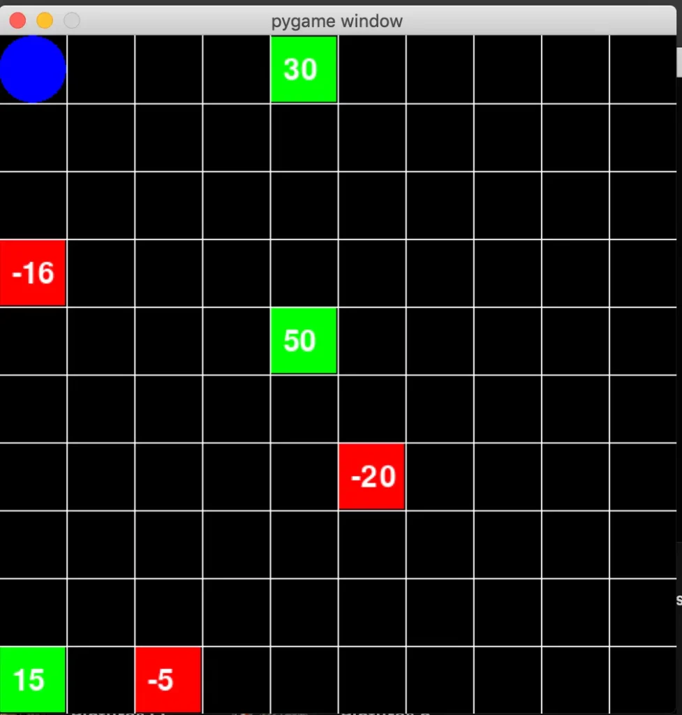
previous figure shows a sample maze environment for a reinforcement learning.

How Reinforcement learning works:

In reinforcement learning (RL), an agent acts in a given environment, is rewarded or punished for those actions, and then modifies its behaviour accordingly. In order to optimize the cumulative reward, this loop assists the agent in making better decisions over time.

There are some essential components in Reinforcement learning process.

Policy
Reward function
Value function
environment model

Types of Reinforcement learning:

There are two types of reinforcement learning models in modern world.

positive reinforcement learning:

When an event that results from a specific behavior strengthens and increases the frequency of that behavior, this is known as positive reinforcement. To put it another way, it influences behavior in a favorable way.

Pros: Maximizes performance, helps sustain change over time.

Cons: Overuse can lead to excess states that may reduce effectiveness.

negative reinforcement learning:

The strengthening of behavior as a result of a negative circumstance being avoided or prevented is known as negative reinforcement.

Pros: Increases behavior frequency, ensures a minimum performance standard.

Cons: It may only encourage just enough action to avoid penalties.

There are major steps in the Reinforcement learning process.

Markov decision process:

Through interaction with its surroundings, the reinforcement learning agent gains knowledge about an issue. Information about its current condition is provided by the environment. The agent then decides which action or actions to perform based on that information. The agent is motivated to repeat that behavior in a comparable future situation if it receives a reward signal from the environment. For each subsequent new state, this procedure is repeated. The agent gradually learns to act in the environment in a way that achieves a predetermined objective through rewards and penalties.

CartPole Game in Reinforcement learning:

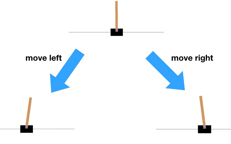
Now let’s talk about one of the most classic problems/use cases in Reinforcement learning called ‘Cartpole environment’. To resolve the problem, we are using the OpenAI GYM library. The concept is actually old. There is a pole in balance and we must keep the pole away from falling over. In this case, the autonomous agent must move a cart either left or right to prevent the pole from falling over and keep the balance.

Now let’s deep dive into the game.

rewards:

Just like any other autonomous agent, The agent we are using for solving this classic game is using a reward system to manage it’s actions against state. It have a understanding that the more time it can keep the pole from falling, the more points/rewards it is getting. By receiving or reducing a point, the agent understand whether the action it took is good or bad. Based on that, the agent will try to optimize and pick the right action. Note that, the game is over when the pole exceeds 12-degree angle or the cart is going out of the screen.

states:

The current condition the cartpole is on is generally known as the current state of agent. There are multiple types of states in reinforcement learning including current state, previous state, next state and end state. Depending on the action we take, it can lead to different other states from current state. Suppose the pole is starting straight, if we go left, the pole is mostly to go right, which is a new state. Therefore, during each time-step, any action we make will always lead to a different state.

Following is a sample codebase for CartPole environment problem solving.

import gym
import numpy as np
import warnings

# Suppress specific deprecation warnings
warnings.filterwarnings("ignore", category=DeprecationWarning)

# Load the environment with render mode specified
env = gym.make('CartPole-v1', render_mode="human")

# Initialize the environment to get the initial state
state = env.reset()

# Print the state space and action space
print("State space:", env.observation_space)
print("Action space:", env.action_space)

# Run a few steps in the environment with random actions
for _ in range(10):
    env.render()  # Render the environment for visualization
    action = env.action_space.sample()  # Take a random action
    
    # Take a step in the environment
    step_result = env.step(action)
    
    # Check the number of values returned and unpack accordingly
    if len(step_result) == 4:
        next_state, reward, done, info = step_result
        terminated = False
    else:
        next_state, reward, done, truncated, info = step_result
        terminated = done or truncated
    
    print(f"Action: {action}, Reward: {reward}, Next State: {next_state}, Done: {done}, Info: {info}")
    
    if terminated:
        state = env.reset()  # Reset the environment if the episode is finished

env.close()  # Close the environment when done

What is Q-learning:

A model-free reinforcement learning technique called Q-learning is used to teach agents—computer programs—to interact with their surroundings and make the best choices possible. It enables the agent to experiment with various activities and determine which ones produce better results. To ascertain which behaviors result in rewards (positive outcomes) or punishments (negative outcomes), the agent employs trial and error.

By updating a Q-table, which contains Q-values that indicate the expected rewards for performing specific actions in specified situations, it gradually enhances its decision-making.

following are the major components of Q-learning process.

Q-value:

Q-values represent the expected rewards for taking an action in a specific state. These values are updated over time using the Temporal Difference (TD) update rule.

Rewards and episodes:

The agent moves through different states by taking actions and receiving rewards. The process continues until the agent reaches a terminal state, which ends the episode.

Greedy policy:

The ϵ-greedy policy helps the agent decide which action to take based on the current Q-value.

Q(S,A)←Q(S,A)+α(R+γQ(S’,A’)–Q(S,A)

the previous formula is used to identify/update the Q-value.

S is the current state.
A is the action taken by the agent.
S’ is the next state the agent moves to.
A’ is the best next action in state S’.
R is the reward received for taking action A in state S.
γ (Gamma) is the discount factor, which balances immediate rewards with future rewards.
α (Alpha) is the learning rate, determining how much new information affects the old Q-values.

following are the procedures in Q-learning process.

Initialization: The agent starts with an initial Q-table, where Q-values are typically initialized to zero.
Exploration: The agent chooses an action based on the ϵ-greedy policy (either exploring or exploiting).
Action and Update: The agent takes the action, observes the next state, and receives a reward. The Q-value for the state-action pair is updated using the TD update rule.
Iteration: The process repeats for multiple episodes until the agent learns the optimal policy.

A Q-table:

In essence, the Q-table is a memory structure in which the agent keeps track of the behaviors that in each condition result in the highest rewards. It is a table of Q-values that show how well the agent comprehends its surroundings. The Q-table is updated by the agent as it investigates and gains knowledge from its interactions with the surroundings. By displaying which activities are most likely to result in better rewards, the Q-table assists the agent in making well-informed decisions.

An example for implementing Q-learning:

first we must identify/define the environment.

import numpy as np

n_states = 16  
n_actions = 4  
goal_state = 15  

Q_table = np.zeros((n_states, n_actions))

Set up the environment parameters including the number of states and actions and initialize the Q-table. In this each state represents a position and actions move the agent within this environment.

Then as the second step of this process, we need to set the necessary parameters.

learning_rate = 0.8
discount_factor = 0.95
exploration_prob = 0.2
epochs = 1000

Now we can implement the Q-learning algorithm into the program.

for epoch in range(epochs):
    current_state = np.random.randint(0, n_states)  
    while current_state != goal_state:
        if np.random.rand() < exploration_prob:
            action = np.random.randint(0, n_actions)  
        else:
            action = np.argmax(Q_table[current_state])  

        next_state = (current_state + 1) % n_states

        reward = 1 if next_state == goal_state else 0

        Q_table[current_state, action] += learning_rate * \
            (reward + discount_factor *
             np.max(Q_table[next_state]) - Q_table[current_state, action])

        current_state = next_state

finally we must get results as the output from algorithm.

print("Learned Q-table:")
print(Q_table)

Deep Q-Learning (DQN):

Deep Q-learning is an advanced algorithmic structure than traditional Q-learning algorithm. It is an extension of the basic Q-Learning algorithm, which uses deep neural networks to approximate the Q-values. Traditional Q-Learning works well for environments with a small and finite number of states, but it struggles with large or continuous state spaces due to the size of the Q-table. Deep Q-Learning overcomes this limitation by replacing the Q-table with a neural network that can approximate the Q-values for every state-action pair.

Now let’s discuss the major concepts behind the Deep-Q-learning process.

Q-function approximation:

Instead of using a table to store Q-values for each state-action pair, DQN uses a neural network to approximate the Q-values. The input to the network is the state, and the output is a set of Q-values for all possible actions.

Experience replay:

To stabilize the training, DQN uses a memory buffer (replay buffer) to store experiences (state, action, reward, next state). The network is trained on random mini-batches of experiences from this buffer, breaking the correlation between consecutive experiences and improving sample efficiency.

Target Network:

DQN introduces a second neural network, called the target network, which is used to calculate the target Q-values. This target network is updated less frequently than the main network to prevent rapid oscillations in learning.

Building a Sample Deep-Q-Learning program:

We are now going to build a Deep-Q-learning algorithm that can solve the Cartpole problem.

import gym
import torch
import torch.nn as nn
import torch.optim as optim
import random
import numpy as np
from collections import deque

# Create the CartPole environment
env = gym.make("CartPole-v1")

# Neural network model for approximating Q-values
class DQN(nn.Module):
    def __init__(self, input_dim, output_dim):
        super(DQN, self).__init__()
        self.fc1 = nn.Linear(input_dim, 128)
        self.fc2 = nn.Linear(128, 128)
        self.fc3 = nn.Linear(128, output_dim)
    
    def forward(self, x):
        x = torch.relu(self.fc1(x))
        x = torch.relu(self.fc2(x))
        return self.fc3(x)

# Hyperparameters
learning_rate = 0.001
gamma = 0.99
epsilon = 1.0
epsilon_min = 0.01
epsilon_decay = 0.995
batch_size = 64
target_update_freq = 1000
memory_size = 10000
episodes = 1000

# Initialize Q-networks
input_dim = env.observation_space.shape[0]
output_dim = env.action_space.n
policy_net = DQN(input_dim, output_dim)
target_net = DQN(input_dim, output_dim)
target_net.load_state_dict(policy_net.state_dict())
target_net.eval()

optimizer = optim.Adam(policy_net.parameters(), lr=learning_rate)
memory = deque(maxlen=memory_size)

# Function to choose action using epsilon-greedy policy
def select_action(state, epsilon):
    if random.random() < epsilon:
        return env.action_space.sample()  # Explore
    else:
        state = torch.FloatTensor(state).unsqueeze(0)
        q_values = policy_net(state)
        return torch.argmax(q_values).item()  # Exploit

# Function to optimize the model using experience replay
def optimize_model():
    if len(memory) < batch_size:
        return
    
    batch = random.sample(memory, batch_size)
    state_batch, action_batch, reward_batch, next_state_batch, done_batch = zip(*batch)

    state_batch = torch.FloatTensor(state_batch)
    action_batch = torch.LongTensor(action_batch).unsqueeze(1)
    reward_batch = torch.FloatTensor(reward_batch)
    next_state_batch = torch.FloatTensor(next_state_batch)
    done_batch = torch.FloatTensor(done_batch)

    # Compute Q-values for current states
    q_values = policy_net(state_batch).gather(1, action_batch).squeeze()

    # Compute target Q-values using the target network
    with torch.no_grad():
        max_next_q_values = target_net(next_state_batch).max(1)[0]
        target_q_values = reward_batch + gamma * max_next_q_values * (1 - done_batch)

    loss = nn.MSELoss()(q_values, target_q_values)

    optimizer.zero_grad()
    loss.backward()
    optimizer.step()

# Main training loop
rewards_per_episode = []
steps_done = 0

for episode in range(episodes):
    state = env.reset()
    episode_reward = 0
    done = False
    
    while not done:
        # Select action
        action = select_action(state, epsilon)
        next_state, reward, done, _ = env.step(action)
        
        # Store transition in memory
        memory.append((state, action, reward, next_state, done))
        
        # Update state
        state = next_state
        episode_reward += reward
        
        # Optimize model
        optimize_model()

        # Update target network periodically
        if steps_done % target_update_freq == 0:
            target_net.load_state_dict(policy_net.state_dict())

        steps_done += 1

    # Decay epsilon
    epsilon = max(epsilon_min, epsilon_decay * epsilon)
    
    rewards_per_episode.append(episode_reward)

# Plotting the rewards per episode
import matplotlib.pyplot as plt
plt.plot(rewards_per_episode)
plt.xlabel('Episode')
plt.ylabel('Reward')
plt.title('DQN on CartPole')
plt.show()

Modern day applications of Q-learning:

There are several fields and industries we are using Q-learning and Deep-Q-learning algorithmic structures today including:

Video game development
robotic system control
autonomous vehicles and robots
Finance
Healthcare
Traffic management
Algorithmic Trading

There are several industries and fields. specially many experts believe that reinforcement learning is a major component in creating AGI (Artificial general Intelligence).

Vishwa GW